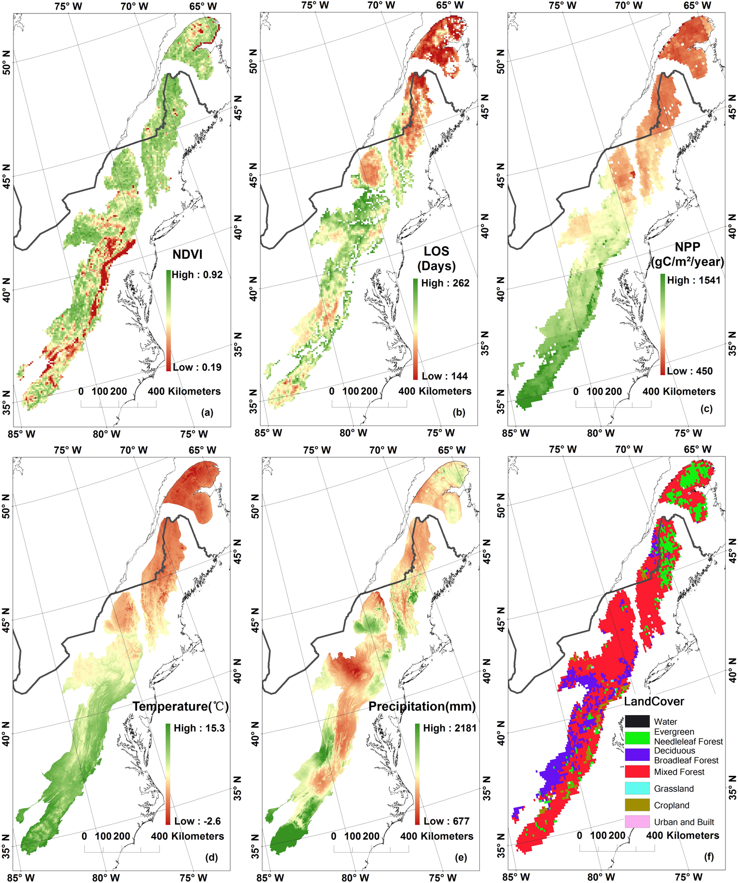
1.

Introduction

The Appalachian Mountains, also known as the Appalachians, are a system of mountains in eastern North America. They run from central Alabama to the New England region of the northeast United States and extend into sections of Quebec, New Brunswick, and Newfoundland in Canada. The mountain range forms a natural barrier between the eastern coastal regions and the interior lowlands of northeastern America. The forests of the Appalachians sustain a variety of ecosystems and native biological diversity. The environmental effects and ecosystem functions and services associated with the Appalachians have long been the focus of scientific research in understanding the mountain range as a unique geographic entity and in comparison with different spatial contexts for providing a regional reference and validation.

The Appalachian Trail is an iconic footpath that traverses high-elevation ridges of the Appalachian Mountains. The trail extends over 3500 km across 14 states in the eastern United States from Springer Mountain in northern Georgia to Mount Katahdin in central Maine. The gradients in elevation, latitude, and moisture sustain a rich biological assemblage of temperate zone forest species. The north-south alignment of the Appalachian Trail corridor represents a cross-section mega-transect of the eastern U.S. forests and alpine areas and provides a barometer for early detection of undesirable changes in the natural resources, such as development encroachment, acid precipitation, invasions of exotic species, and climate change impacts.^1,2

Climate change studies reveal the effects of global warming on the growing season of terrestrial vegetation at middle and high latitudes.^3,4 Over the 20th century, the global average surface temperature increased $0.6\pm 0.2°\mathrm{C}$. Observable warming occurred between 1976 and 2000, and temperatures are projected to increase^5,6 by 1.4°C to 5.8°C from 1990 to 2100. Tracking variations in landscape dynamics provides an understanding of the changing environment, the impacts and threats caused by changes, and the likely trends in the future for natural resources and associated ecosystems.⁷ Time series remote sensing data provide necessary observations in revealing patterns of landscape dynamics either by abrupt change or gradual variations.

The normalized difference vegetation index (NDVI) has been effectively used for monitoring vegetation dynamics. Consistent and long time-series NDVI data are important for analysis of vegetation responses to global change in terrestrial ecosystems.⁸ The Global Inventory Monitoring and Modeling Studies (GIMMS) NDVI dataset derived from Advanced Very High Resolution Radiometer (AVHRR) has been broadly used for studying vegetation activity on regional and global scales.

Phenology studies have long been reported in different domains, such as climate change.⁹ biodiversity,¹⁰ wildlife ecology,¹¹ snow dynamics,¹² fire effects,¹³ and crops.¹⁴ Land surface phenology (LSP) is one of the measures of landscape dynamics. It reflects the response of vegetated surfaces to seasonal and annual changes in the climatic and hydrologic cycle. LSP is strongly linked to climatic factors.¹⁵ It has been broadly studied in the context of ecosystem responses to climate change¹⁶ and for monitoring and understanding global change in vegetation lifecycle events. Because of spatial resolution of remote sensing data, LSP is described as an indicator of mixtures of land covers and is distinct from traditional notion of species-centric phenology, such as seasonal flowering or budburst.^17,18 Because LSP is based on remote sensing observations at regional and global scales, it serves as a key biological indicator for detecting the response of terrestrial ecosystems to climatic variation.

LSP metrics are primarily based on time series images of vegetation indices from optical sensors such as AVHRR, spot-vegetation (VGT), and moderate resolution imaging spectroradiometer (MODIS). These metrics typically retrieve the time of the onset of greenness as the start of the season (SOS), onset of senescence or time of end of greenness as the end of the season (EOS), timing of the maximum of the growing season by peak vegetation indices, and the length of growing season (LOS) or duration of greenness. An increasing number of studies have reported the shifts in timing and length of the growing season based on phenology, satellite data, and climatological studies.⁶

Net primary production (NPP) plays an important role in the Earth surface system’s health¹⁹ and the terrestrial carbon cycle.^20,21 NPP and its response to climate change have been the focus of global change research.²² Studies have been conducted based on historical datasets.^23–32 Recent climatic changes have enhanced plant growth in northern middle and high latitudes.³¹ Various NPP models have been developed to analyze NPP response to climate change.^32–42 Regional scale carbon cycle processes and climate patterns provide indications of potential responses and feedback to climate change.⁴³

Other studies showed that temperatures across the northeastern United States have been increasing steadily since the 1970s. A wide range of indicators in the Northeast have already been observed to be responsive to the changes, which in turn have the potential to impact urban and rural life, agriculture, industry, tourism, and natural ecosystems.⁴⁴ The U.S. Global Change Research Program reported that the annual average temperature in the Northeast has increased by 1.1°C, with winter temperatures rising twice that much, since 1970. At the same time, warming has resulted in many other climate-related changes, including more frequent days with temperatures above 32.2°C, longer growing seasons, increased heavy precipitation, more winter precipitation falling as rain instead of snow, reduced snowpack, earlier breakup of winter ice on lakes and rivers, and earlier spring snowmelt resulting in earlier peak river flows and rising sea surface temperatures and sea levels.⁴⁵ Projections along the Appalachian Trail corridor area showed a steady temperature increase ranging from 2°C to 6°C by the end of the 21st century. Precipitation, however, did not show any significant trend or decadal variation.⁴⁶

Therefore, the objective of this study is to investigate the patterns and trends of NDVI, LSP, and NPP of the Appalachian Mountains regions and make comparisons of those variables with different scales of spatial contexts using time series GIMMS and Global Production Efficiency Model (GloPEM) datasets.^37,47

2.

Materials and Methods

2.1.

Study Areas

The selected Appalachian Mountains regions consist of four provinces of ecoregions in the United States and Canada covering a latitudinal range between $34°4^{\prime }\mathrm{N}$ and $49°{15}^{\prime }\mathrm{N}$ and $\mathrm{406,944}{\mathrm{km}}^2$ in area (Fig. 1). The provinces of ecoregions include the Adirondack-New England Mixed Forest-Coniferous Forest-Alpine Meadow Province, the Eastern Broadleaf Forest Province, and the Central Appalachian Broadleaf Forest-Coniferous Forest-Meadow Province in the United States⁴⁸ and a section of the Eastern Canadian Forests.

Fig. 1

The study area consists of four provinces of ecoregions along the Appalachian Mountains in the eastern United States and southeastern Canada. The selected Appalachian Mountains ecoregion provinces include (A) Eastern Canadian Forests, (B) Adirondack-New England Mixed Forest-Coniferous Forest-Alpine Meadow Province, (C) Eastern Broadleaf Forest Province, and (D) Central Appalachian Broadleaf Forest-Coniferous Forest-Meadow Province. North America and an Appalachian Trail corridor area are selected for the comparative studies.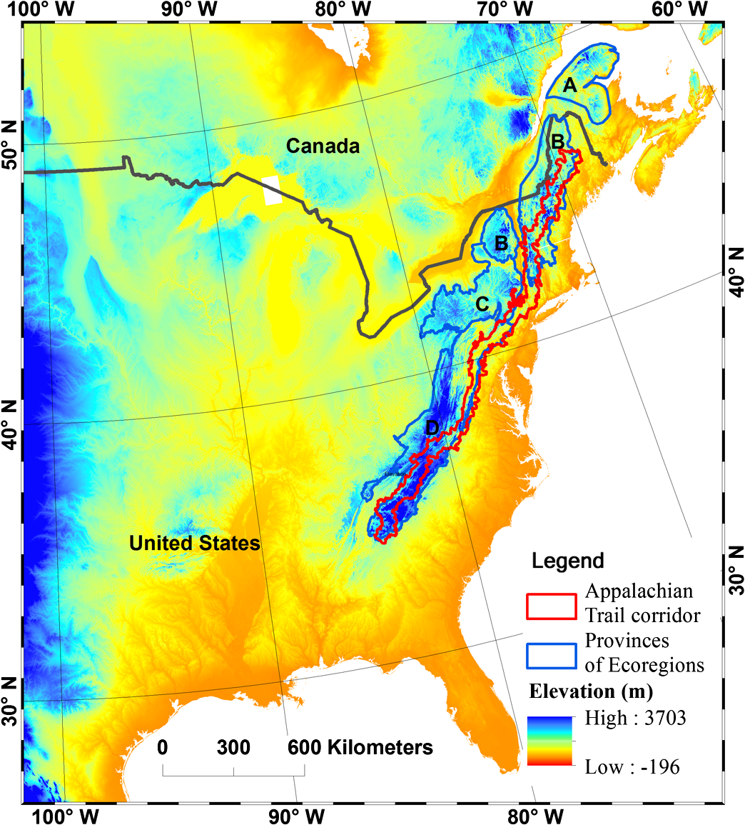

The Adirondack-New England Mixed Forest-Coniferous Forest-Alpine Meadow Province has a modified continental climatic regime with long, cold winters and warm summers. Annual precipitation is evenly distributed. The landscape is mountainous and was previously glaciated. Forest vegetation is a transition between boreal on the north and broadleaf deciduous to the south. The Eastern Broadleaf Forest Province has a continental-type climate of cold winters and warm summers. Annual precipitation is greater during the summer. Topography is variable, ranging from plains to low hills of low relief along the Atlantic coast. Interior areas are high hills to semi-mountainous, parts of which were glaciated. Vegetation is characterized by tall, cold-deciduous broadleaf forests. The Central Appalachian Broadleaf Forest-Coniferous Forest-Meadow Province is a moderately dissected plateau of irregular plains and open hills. Geologic formations are mostly marine deposits of limestones, shales, and sandstone. The existing land cover type is mainly agricultural and urban. Small areas of natural cover types remain, consisting of forests of oak-hickory, maple-beech-birch, and oak-gum-cypress cover types. The Eastern Canadian Forests are characterized by forested land in eastern Quebec, much of Newfoundland, the highlands of New Brunswick, and Cape Breton Island, Nova Scotia. The climate ranges from high and mid-boreal and perhumid mid-boreal to Oceanic, Atlantic, and maritime mid-boreal. Summers are generally cool, with average temperatures ranging from 8.5°C in the north to 14.5°C in the south. Winter temperatures vary according to the proximity to the ocean and continental landmass.

In order to reveal the differences and similarities of NDVI, SOS, and NPP in the Appalachian Mountains regions, we compared the variables in different spatial scales with North America and the Appalachian Trail corridor area (Fig. 1), and in different latitudinal ranges from 30°N to 40°N and 40°N to 50°N in North America.

3.

Results

3.1.

Spatial Pattern Of NDVI, LSP, and NPP

Figure 2 illustrates spatial patterns of the mean value of peak NDVI, LSP, NPP, Temperature, Precipitation, and Land Cover. The peak NDVI, LSP, and NPP represent the maximum value of the year and were obtained using the MVC method. The mean peak NDVI, LSP, and NPP were obtained similarly. Land cover types were considered in obtaining the spatial variation of NDVI, as shown in Fig. 2(a) and 2(f). For example, forests are mainly distributed in humid climatic zones of the Appalachian Mountains⁷³ and therefore possess high NDVI values. At pixel scale, the data illustrate spatial dynamics of LOS of the Appalachian Mountains between 1982 and 2006. The spatial variation indicates that the average LOS varied from 144 to 262 days, and extended LOS was observed in low-latitude areas, as shown in Fig. 2(b). The patterns indicate that LOS increased from northeast to southwest in these areas. Spatial pattern reveals that LOS was more responsive to the variation of temperature [Fig. 2(d)] than to precipitation [Fig. 2(e)]. Annual mean NPP ranged from 450 to $\mathrm{1,541}\mathrm{g}{\mathrm{Cm}}^{-2}{\mathrm{yr}}^{-1}$ [Fig. 2(c)] in the Appalachian Mountains over the 20 years from 1991 to 2000. NPP values reflected the latitudinal effects from southwest to northeast at 34°N to 40°N, 40°N to 45°N, and 45°N to 50°N. Areas with low NPP were found in the high-latitude regions, consistent with the changes in temperature [Fig. 2(d)]. The pattern of temperature variation showed a decreasing trend from southwest to northeast. The mean temperature showed high values from 34°N to 40°N, medium values from 40°N to 45° N, and low values from 45°N to 50°N. The precipitation was highest with $\mathrm{2,181}\mathrm{mm}/\text{year}$ in the low-latitude regions, as shown in Fig. 2(e). In the southwestern region, the NPP, temperature, and precipitation measures were higher than those in other regions. A combination of higher temperature and precipitation contributes to high NPP in the southwestern region of the Appalachian Mountains.

Fig. 2

The spatial patterns of mean peak NDVI, LSP, NPP, Temperature, Precipitation, and Land Cover of the studied Appalachian Mountains regions.

3.2.

Trends Of NDVI, LSP, and NPP

The trend of NDVI in the Appalachian Mountains regions varied from $-0.012$ to 0.0056 units. The declining trends of peak NDVI occurred in the Appalachian Mountains, particularly in the central regions [Fig. 3(a)]. Only the section area within the Eastern Canadian Forests showed increasing trends of peak NDVI.

Fig. 3

Trends in peak NDVI, LOS, and NPP within the selected Appalachian Mountains regions from 1982 to 2006.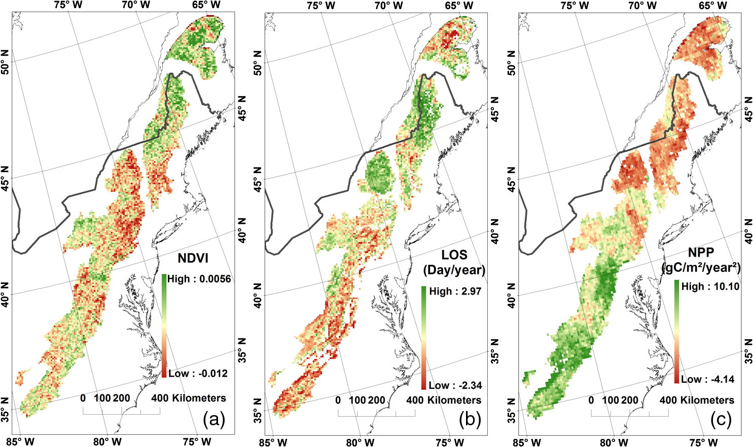

Spatial variations in LOS trends indicate that LOS varied between $-2.34$ days (decreasing) to 2.97 days (increasing) per year from 1982 to 2006 over the Appalachian Mountains regions [Fig. 3(b)]. The decreasing trends ($<-1\text{days}{\mathrm{yr}}^{-1}$) were mainly found in the Central Appalachian Broadleaf Forest-Coniferous Forest-Meadow Province and the Eastern Canadian Forests. Positive LOS trends mainly occurred in the Adirondack-New England Mixed Forest-Coniferous Forest-Alpine Meadow Province, as shown in Fig. 3(b).

We calculated the trends in NPP at the pixel level (8 km) from 1981 to 2000 using linear least squares. These calculations are shown in Fig. 3(c). Positive and negative NPP trends were found across the Appalachian Mountains regions. Observable increases occurred in the Central Appalachian Broadleaf Forest-Coniferous Forest-Meadow Province and the Northeastern Mixed Forest Province. A decrease in NPP occurred in the northeast, and an increased trend was observed in the southwest of the Appalachian Mountains.

3.3.

Comparison of Appalachian Mountains with Different Spatial Contexts

The NDVI data were calculated for vegetated area only. For Figs. 4Fig. 5–6, the straight lines were generated using the method of linear least squares. Significant decrease in annual peak NDVI was observed in the Appalachian Mountains, as well as the Appalachian Trail corridor area (Fig. 4). The average slope in the Appalachian Mountains was a $-0.0018$ ($R^2=0.55$, $P<0.0001$) NDVI unit decrease per year during the 25 years from 1982 to 2006. For the Appalachian Trail corridor area, the average slope was a $-0.0022$ ($R^2=0.62$, $P<0.0001$) NDVI unit decrease per year over the 25 years. However, there was no observable trend in North America or in the selected latitudinal ranges from 30°N to 40°N and from 40°N to 50°N (Fig. 4 and Table 1).

Fig. 4

The interannual variability of NDVI for the Appalachian Mountains, North America, the 30°N–40°N range in North America, the 40°–50°N range in North America, and the Appalachian Trail corridor area between 1982 and 2006.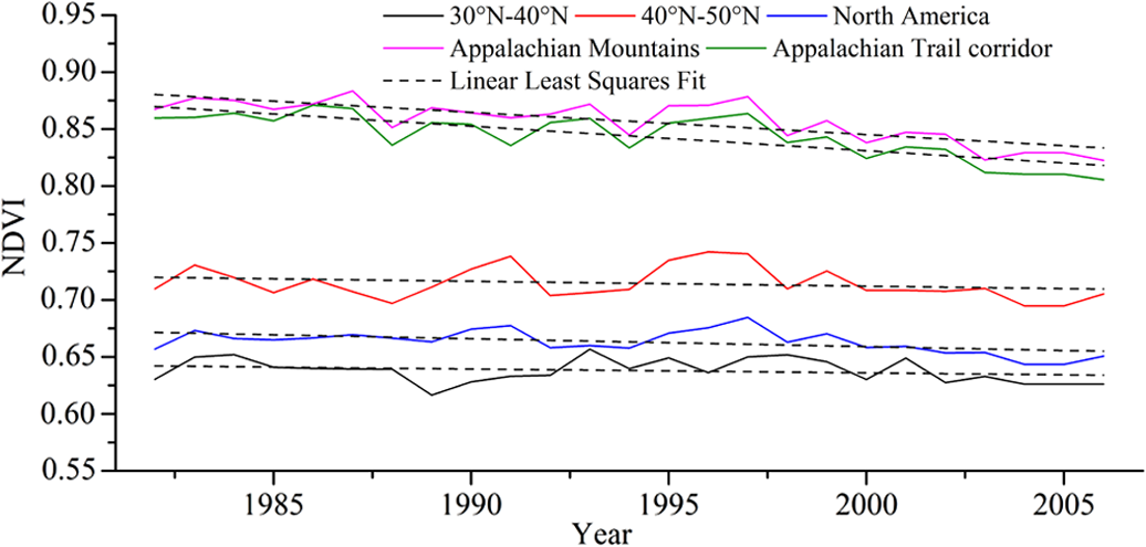

Fig. 5

The variation of LOS for the Appalachian Mountains, North America, the 30°N–40°N range in North America, the 40°N–50°N range in North America, and the Appalachian Trail corridor area.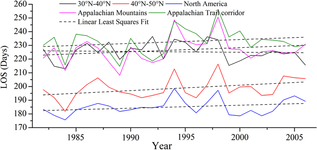

Fig. 6

The variation in NPP for the Appalachian Mountains, North America, the 30°N–40°N range in North America, the 40°N–50°N range in North America, and the Appalachian Trail corridor area.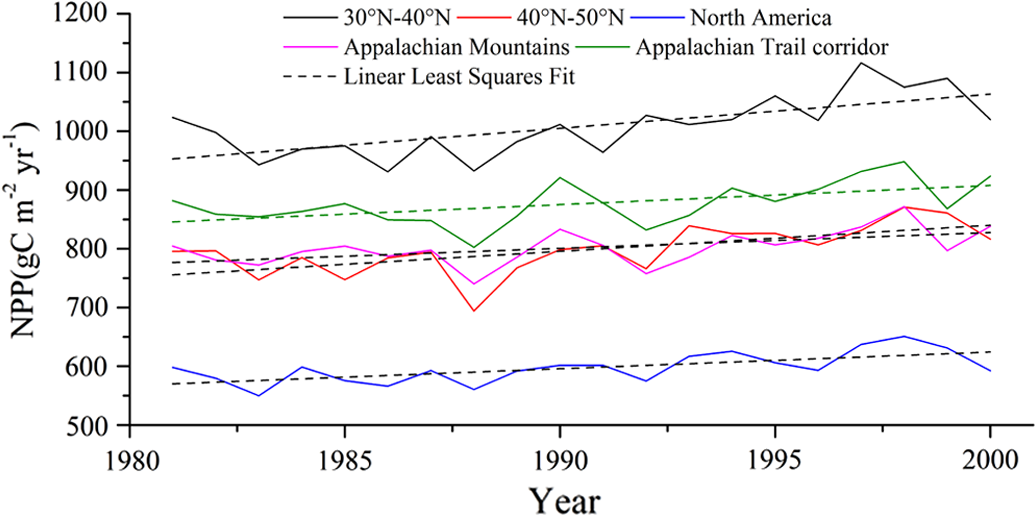

Table 1.

The parameters of NDVI, LOS, and NPP

	Parameter	30°N–40°N	40°N–50°N	North America	Appalachian Mountains	Appalachian Trail Corridor
NDVI 1982–2006	Max	0.6567	0.7404	0.6422	0.8865	0.8715
	Min	0.6167	0.6931	0.6032	0.8267	0.8047
	Mean	0.6380	0.7135	0.6208	0.8603	0.8430
	Slope	$-0.0004$	$-0.0004$	$-0.0004$	$-0.0018$	$-0.0022$
	$R^2$	0.0194	0.0132	0.0432	0.5505	0.6202
	$P$	0.2369	0.2622	0.1624	0.0000	0.0000
LOS 1982–2006	Max	237	216	199	251	256
	Min	213	182	176	208	215
	Mean	225	199	185	227	233
	Slope	$-0.0588$	0.3937	0.2167	0.3000	0.2841
	$R^2$	$-0.0394$	0.1126	0.0396	0.0149	0.0085
	$P$	0.7651	0.0561	0.1718	0.2550	0.2836
NPP 1981–2000	Max	1117	871	651	872	948
	Min	931	694	550	740	802
	Mean	1009	797	597	802	877
	Slope	5.7980	4.4441	2.8544	2.6820	3.2669
	$R^2$	0.4347	0.3731	0.3879	0.2399	0.2485
	$P$	0.0009	0.0025	0.0020	0.0165	0.0147

The prolonged LOS was $0.3\text{day}{\mathrm{yr}}^{-1}$ over the entire Appalachian Mountains, $0.39\text{day}{\mathrm{yr}}^{-1}$ in latitudinal zone from 40°N to 50°N, $0.02\text{day}{\mathrm{yr}}^{-1}$ in North America, and $0.28\text{day}{\mathrm{yr}}^{-1}$ in the Appalachian Trail corridor area. However, the LOS trend was shortened by $0.06\text{day}{\mathrm{yr}}^{-1}$ in latitudes from 30°N to 40°N. Although there was no indication of a significant trend in LOS in any region during the study time periods, abnormal values in some years (e.g., 1998 and 1999) were observable against the calculated mean values and are shown in Fig. 5.

We calculated the annual mean NPP values for the Appalachian Mountains, North America, and the Appalachian Trail corridor area (Fig. 6 and Table 1). The average NPP values were 1,008, 797, 597, 802, and $876\mathrm{g}{\mathrm{Cm}}^{-2}{\mathrm{yr}}^{-1}$, in the 30°N–40°N range, the 40–50°N range, North America, the Appalachian Mountains, and the Appalachian Trail corridor area, respectively. The increasing trend in NPP was observed for all the regions during the 20-year period (Fig. 6). The NPP increased $2.68\mathrm{g}{\mathrm{Cm}}^{-2}{\mathrm{yr}}^{-2}$ ($R^2=0.24$, $P=0.016$) from 1982 to 2006 in Appalachian Mountains. The trends in NPP showed an increase of $5.80\mathrm{g}{\mathrm{Cm}}^{-2}{\mathrm{yr}}^{-2}$ ($R^2=0.43$, $P<0.0009$) in the 30°N–40°N range, $4.44\mathrm{g}{\mathrm{Cm}}^{-2}{\mathrm{yr}}^{-2}$ ($R^2=0.37$, $P=0.0025$) in the 40°N–50°N range, $2.85\mathrm{g}{\mathrm{Cm}}^{-2}{\mathrm{yr}}^{-2}$ ($R^2=0.39$, $P=0.002$) in North America, and $2.17\mathrm{g}{\mathrm{Cm}}^{-2}{\mathrm{yr}}^{-2}$ ($R^2=0.25$, $P=0.015$) in the Appalachian Trail corridor.

4.

Conclusions and Discussion

This study revealed the spatial and temporal variations and trends in landscape dynamics, LSP, and NPP in the study area. The comparisons examined the Appalachian Mountains as a unique geographic entity and their topographic and elevation effects in the spatial context. Our conclusions are as follows.

The peak NDVI values decreased significantly in the Appalachian Mountains and the Appalachian Trail corridor area (Fig. 4). Both trends possessed higher negative slopes than those in the 30°N–40°N and 40°N–50°N latitudinal zones and North America. The mean peak NDVI values were 0.86 in the Appalachian Mountains and 0.84 in the Appalachian Trail corridor, higher than those of North America. Other studies have suggested that the average annual peak NDVI presented a declining trend over many protected areas in North America.⁵⁰ Given that neither temperature nor precipitation showed a correlation with NDVI, this may imply that the observed decrease in NDVI was mainly driven by the combination of urban expansion and outbreaks of hemlock wooly adelgids (Adelges tsugae)^74–76 and other insect pests. Consistent with the patterns observed in the AVHRR GIMMS data along the Appalachian Trail corridor, analyses using other types of remote sensing data have shown a decrease in forest cover in the eastern U.S., mainly due to the growth of urban areas since the 1970s.^7,77–79

There are different results from different methods for calculation of LSP parameters.⁶⁴ For example, the results from four methods were very much different. The SOS calculated by the moving average method was the lowest, and the EOS value was the highest, but the derivative method delivered the highest SOS value and the lowest EOS value.

A reported LSP study suggested that the EOS in North America was delayed by 8.1 days per decade from 1982 to 1999 and by 1.3 days per decade from 2000 to 2008.⁸⁰ Another study reported that SOS advanced by approximately 8 days, EOS was delayed by 4 days, and LOS increased by 12 days in North America from 1982 to 1999.⁸¹ The results of this study suggested that LOS in the Appalachian Mountains advanced 7.5 days from 1982 to 2006. The longest annual mean LOS value (233 days) was observed in the Appalachian Trail corridor area, and the second longest LOS value (227 days) was observed in the Appalachian Mountains regions. The mean LOS in the latitudinal range between 40°N and 50°N increased by $0.39\text{days}{\mathrm{yr}}^{-1}$ ($R^2=0.11$, $P=0.056$) from 1982 to 2006; that increase was higher than those in other regions. The overall trend along the Appalachian Mountains, despite local variations, agreed with broader patterns obtained for the Northern Hemisphere and North America. The local variations were caused by topographic and elevation effects, as well as associated land cover types and ecosystems.

To further understand the effect of elevation, we divided the LOS into 20 categories from $-5\mathrm{m}$ to 2,025 m. We found that the LOS was shortened by 1.2 days ($R^2=0.86$, $P<0.001$) for every 100-m increase in elevation. The prolonged LOS was mainly attributed to delayed EOS. This study concluded that the variations and trends of LSP metrics in the Appalachian Mountains were comparable to those obtained for the Appalachian Trail corridor area.⁸² The LOS anomalies in 1987, 1994, and 1998 followed the pattern of warm and cold episodes based on a threshold of $+/-0.5°\mathrm{C}$ for the Oceanic Niño Index (ONI). The reversed LOS patterns correspond to El Niño in 1997 to 1998 and La Niña in 1999 to 2000 events.⁸³ This indicates that LOS is sensitive to climate variations.

NPP modeling studies have documented that terrestrial photosynthetic activity has increased over the past two to three decades in the middle and high latitudes in the Northern Hemisphere.^{28–30,32,84} The mean annual NPP in North America (north of 22°N) was reported as $6.2\mathrm{Pg}\mathrm{C}{\mathrm{yr}}^{-1}$, increasing by $0.028\mathrm{Pg}\mathrm{C}{\mathrm{yr}}^{-2}$ (significant at the 99% level) from 1982 to 1998.²⁸ The results from this study illustrated significant increasing trends of NPP from 1981 to 2000 in all the study regions. The NPP in the Appalachian Mountains increased by $2.68\mathrm{g}{\mathrm{Cm}}^{-2}{\mathrm{yr}}^{-2}$ ($R^2=0.24$, $P=0.017$), a smaller rate than that for North America ($2.85\mathrm{g}{\mathrm{Cm}}^{-2}{\mathrm{yr}}^{-2}$, $R^2=0.39$, $P=0.002$). The largest annual mean NPP value ($1009\mathrm{g}{\mathrm{Cm}}^{-2}{\mathrm{yr}}^{-1}$) and the largest trend increase ($5.8\mathrm{g}{\mathrm{Cm}}^{-2}{\mathrm{yr}}^{-2}$, $R^2=0.43$, $P=0.0009$) were observed in the latitudinal range between 30°N and 40°N. The mean NPP in the Appalachian Trail corridor area increased by $3.23\mathrm{g}{\mathrm{Cm}}^{-2}{\mathrm{yr}}^{-2}$ ($R^2=0.25$, $P=0.015$), which was larger than that for North America and smaller than that for the Appalachian Mountains regions.

While prolonged LOS and increasing trends of annual NPP were observed in the Appalachian Mountains and the Appalachian Trail corridor, peak NDVI showed a decreasing trend. There are many factors that could affect the change of NDVI, LOS, and NPP in different spatial contexts of the study areas. The similar pattern of variations and trends between the Appalachian Trail corridor area and the Appalachian Mountains regions suggested that the Appalachian Trail corridor area can serve as a mega-transect to reflect such variations and trends of the Appalachian Mountains regions.